SGD with Momentum

Gradient Descent Algorithm: 11 Part(s)

Introduction

In the previous post about, we discussed the Stochastic Gradient Descent algorithm. Remember that SGD helps us to minimize the cost function using one random data point at a time. In some cases, it would help us to converge relatively faster and reduces the RAM usage significantly compared to the Vanilla Gradient Descent algorithm.

However, the SGD algorithm has some limitations. It oscillates a lot, still requires a longer time to converge, and sometimes it may not converge at all because not be able to escape the local minima. With the help of Momentum, we can overcome these limitations.

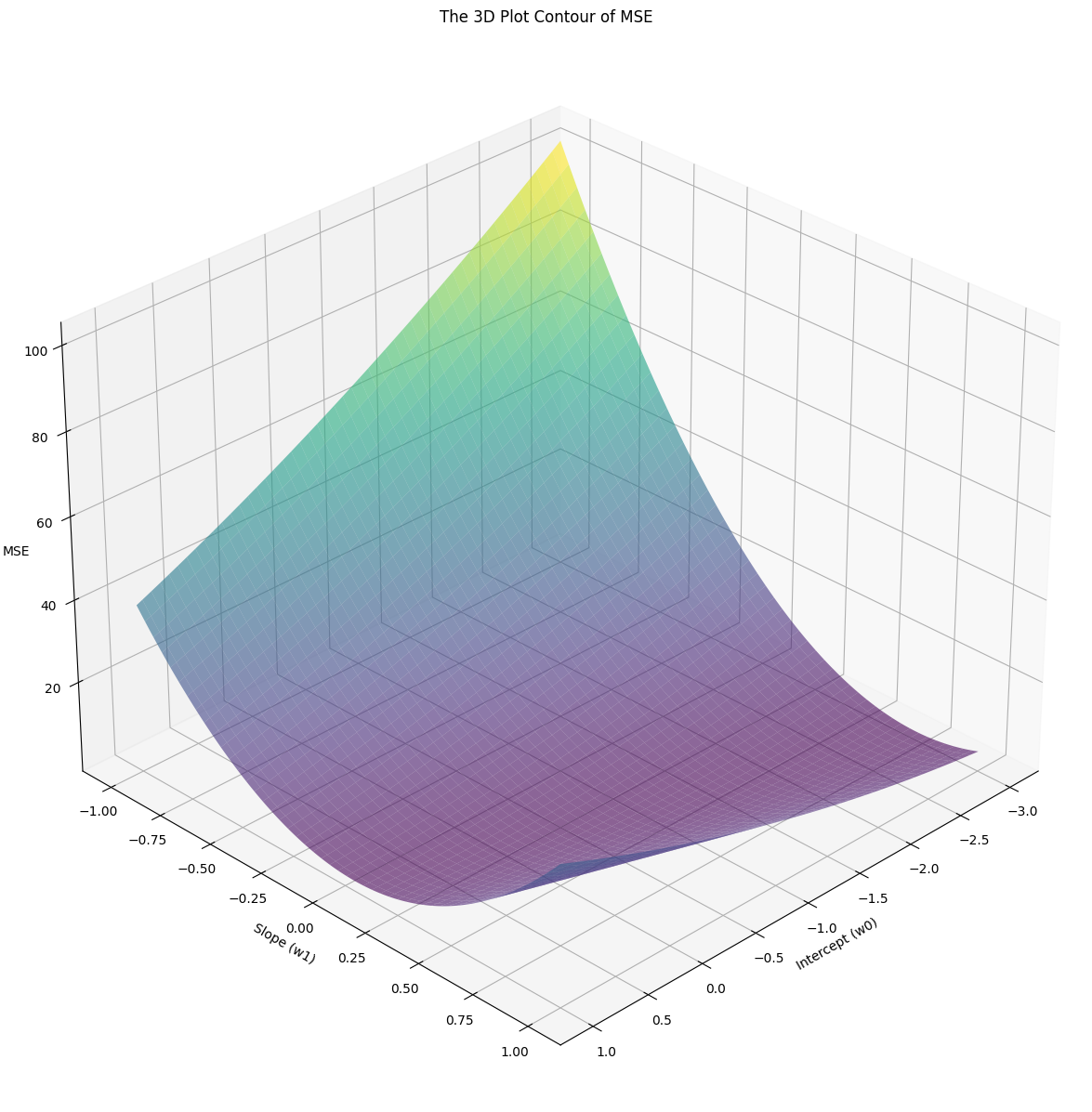The 3D contour of the MSE of Iris Dataset

Imagine rolling a ball down a hill. As it moves, it gains momentum, rolling faster until it reaches its maximum speed. Clearly, the ball's current speed is determined based on it's previous speed. In addition to that, if it's contour is smooth, the ball will roll faster and faster until it reaches the bottom of the hill. If it's contour is rough, the ball will oscillate a lot and reach the bottom of the hill slowly. The same concept applies to SGD with Momentum.

Mathematics of SGD with Momentum

The parameter update rule is expressed as

\begin{aligned} v_{i, t} &= \gamma v_{i, t-1} + \alpha \nabla_{\theta} J(\theta) \\ \theta_i &= \theta_i - v_{i,t} \end{aligned}

where

$v_{i,t}$ is the $i$ -th Momentum vector at time $t$
$\gamma$ is the momentum coefficient
$\alpha$ is the learning rate
$\nabla J(\theta)$ is the gradient of the cost function $J(\theta)$
$\theta_i$ is the $i$ -th parameter

The gradient of the cost function w.r.t. to the intercept $\theta_0$ and the coefficient $\theta_1$ are expressed as the following.

\begin{aligned} \nabla_{\theta_0} J(\theta) &= \frac{\partial}{\partial \theta_0} J(\theta) \\ &= \frac{1}{2} \frac{\partial}{\partial \theta_0} (\hat{y}_i - y_i)^2 \\ &= \hat{y}_i - y_i \end{aligned}

\begin{aligned} \nabla_{\theta_1} J(\theta) &= \frac{\partial}{\partial \theta_1} J(\theta) \\ &= \frac{1}{2} \frac{\partial}{\partial \theta_1} (\hat{y}_i - y_i)^2 \\ &= (\hat{y}_i - y_i)x_i \end{aligned}

Notice that the gradient of the cost function w.r.t. the intercept $\theta_0$ is the error of the prediction.

Since there are two parameters to update, we are going to need two parameter update rules.

\begin{aligned} v_{0, t} &= \gamma v_{0, t-1} + \alpha (\hat{y}_i - y_i) \\ \theta_0 &= \theta_0 - v_{0,t} \end{aligned}

\begin{aligned} v_{1, t} &= \gamma v_{1, t-1} + \alpha (\hat{y}_i - y_i)x \\ \theta_1 &= \theta_1 - v_{1,t} \end{aligned}

With the Momentum coefficient, we smooth out the updates. If gradients point in the same direction, meaning having the same sign (positive or negative), the Momentum vector will take larger steps. If gradients point in different directions, the Momentum coefficient $\gamma$ will help reduce oscillations. In most cases, it is set to $0.9$ .

Implementation of SGD with Momentum

First, determine the prediction error and the gradient of the cost function w.r.t the intercept $\theta_0$ and the coefficient $\theta_1$ .

error = prediction - y[random_index]
t0_gradient = prediction - y[random_index]
t1_gradient = (prediction - y[random_index]) * x[random_index]

Next, we have to update the Momentum vectors. For simplicity, we are not going to store the vector of $\theta_0$ and $\theta_1$ into a list. Instead, we are storing them into separate variables, t0_vector and t1_vector respectively.

\begin{aligned} v_{0, t} &= \gamma v_{0, t-1} + \alpha \nabla_{\theta_0} J(\theta) \\ v_{1, t} &= \gamma v_{1, t-1} + \alpha \nabla_{\theta_1} J(\theta) \\ \end{aligned}

Since the updated t0_vector relies on the previous t0_vector, we need to initialize them to zero outside the loop.

t0_vector, t1_vector = 0.0, 0.0
...
 
for epoch in range(1, epochs + 1):
  ...
  t0_vector = gamma * t0_vector + alpha * t0_gradient
  t1_vector = gamma * t1_vector + alpha * t1_gradient

Finally, update the parameters.

intercept = intercept - t0_vector
coefficient = coefficient - t1_vector

Conclusion

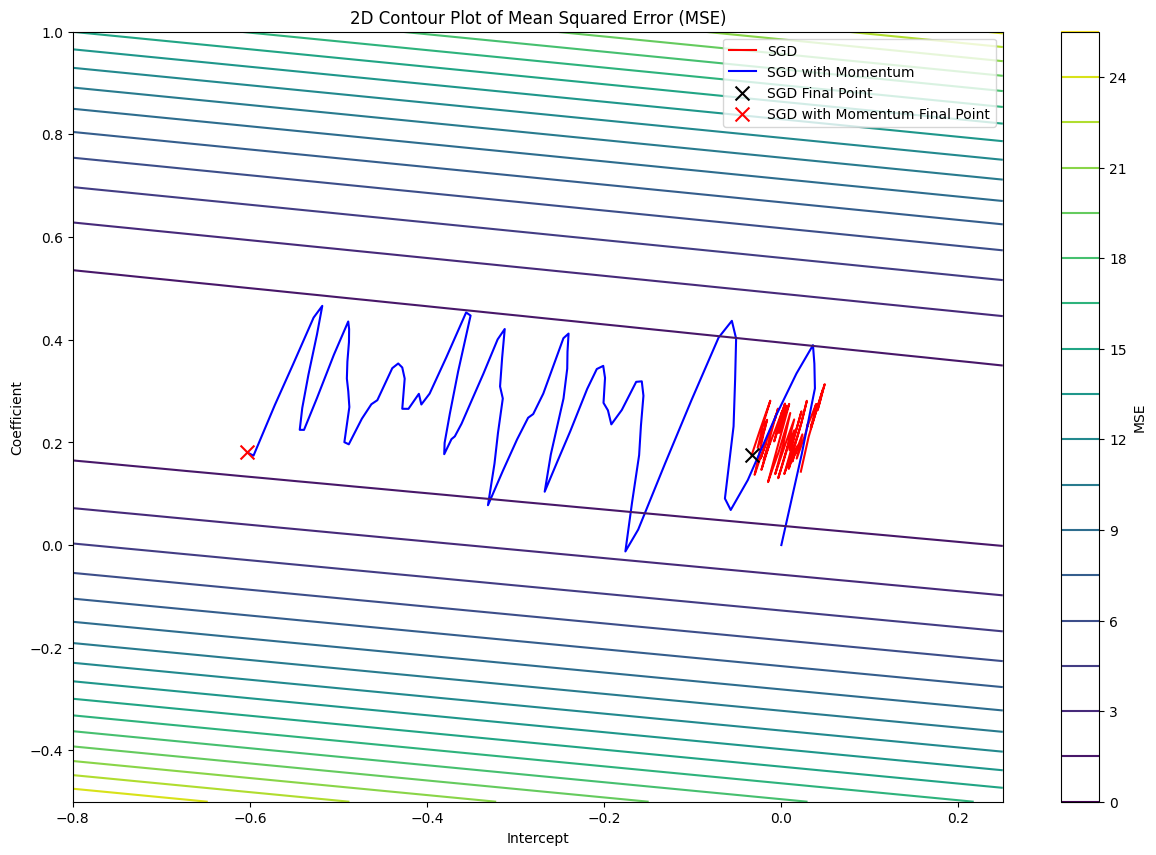The loss function pathway of SGD with and without Momentum

From the image above, we can see that the loss function pathway of SGD with Momentum is much more like a ball rolling down a hill. On the otherhand, Vanilla SGD oscillates a lot while traversing through the valley compared to SGD with Momentum.

Code

def predict(intercept, coefficient, x):
  return intercept + coefficient * x
 
def sgd_momentum(x, y, df, epochs=100, alpha=0.01, gamma=0.9):
  intercept, coefficient = 0.0, 0.0
  t0_vector, t1_vector = 0.0, 0.0
  random_index = np.random.randint(len(features))
  prediction = predict(intercept, coefficient, x[random_index])
  error = ((prediction - y[random_index]) ** 2) / 2
 
  df.loc[0] = [intercept, coefficient, t0_vector, t1_vector, error]
 
  for epoch in range(1, epochs + 1):
    random_index = np.random.randint(len(features))
    prediction = predict(intercept, coefficient, x[random_index])
 
    error = prediction - y[random_index]
    t0_gradient = error
    t1_gradient = error * x[random_index]
 
    t0_vector = gamma * t0_vector + alpha * t0_gradient
    t1_vector = gamma * t1_vector + alpha * t1_gradient
 
    intercept = intercept - t0_vector
    coefficient = coefficient - t1_vector
 
    mse = (error ** 2) / 2
    df.loc[epoch] = [intercept, coefficient, t0_vector, t1_vector, mse]
 
  return df

References

Sebastian Ruder. "An overview of gradient descent optimization algorithms." arXiv:1609.04747 (2016)
Ning Qian. "On the momentum term in gradient descent learning algorithms." Neural Networks (1999)