RMSprop

Gradient Descent Algorithm: 11 Part(s)

Introduction

In the Adadelta post, we have discussed the limitations of the Adagrad algorithm, the rapid decay of the learning rate. Adadelta solves limitation by calculating the average squared of the decayed gradients over time.

RMSprop also solves the limitation of Adagrad just like Adadelta. Unlike Adadelta The only difference is that RMSprop uses the learning rate value, and divides it with the root mean squared of the decayed gradients. This algorithm was proposed independently by Geoffrey Hinton around the same time as Adagrad. However, this algorithm was never published.

Mathematics of RMSprop

The parameter update rule is expressed as

\theta_{t+1} = \theta_t - \frac{\alpha}{\sqrt{E[g^2]_t + \epsilon}} \odot g_t

where

$\theta_t$ is the parameter at time $t$
$\alpha$ is the learning rate
$\sqrt{E[g^2]_t + \epsilon}$ is the root mean squared of the decayed gradients up to time $t$

Collectively, $E[g^2]_t$ , the decayed gradients up to time $t$ , can be expressed as follows:

\begin{aligned} E[g^2]_t &= (0.9 E[g^2]_{t-1} + 0.1g_t^2) + \ldots + (0.9 E[g^2]_{0} + 0.1g_0^2) \end{aligned}

where

E[g^2]_{t-1} = \frac{g_{t-1}^2 + ... + g_0^2}{t-1}

Since there are two parameters, we need determine $g_{0,t}$ is the gradient of the cost function at time $t$ w.r.t. to the intercept $\theta_0$ , and $g_{1,t}$ is the gradient of the cost function at time $t$ w.r.t. to the coefficient $\theta_1$ .

\begin{aligned} g_{0, t} &= \nabla_{\theta_0} J(\theta) \\ &= \frac{\partial}{\partial \theta_0} J(\theta) \\ &= \frac{1}{2} \frac{\partial}{\partial \theta_0} (\hat{y}_i - y_i)^2\\ &= \hat{y}_i - y_i \end{aligned}

\begin{aligned} g_{1, t} &= \nabla_{\theta_1} J(\theta) \\ &= \frac{\partial}{\partial \theta_1} J(\theta) \\ &= \frac{1}{2} \frac{\partial}{\partial \theta_1} (\hat{y}_i - y_i)^2\\ &= (\hat{y}_i - y_i)x_i \end{aligned}

Implementation of RMSprop

First, First, calculate the intercept and the coefficient gradient. Notice that the intercept gradient $g_{t,0}$ is the predicion error.

error = prediction - y[random_index]
new_intercept_gradient = error
new_coefficient_gradient = error * x[random_index]

Second, calculate the running average of the squared gradients $E[g^2]_t$ . $E[g^2]_{t-1}$ can be written as np.mean(df['intercept_gradient'].values ** 2).

mean_squared_intercept = (0.9 * np.mean(df['intercept_gradient'].values ** 2)) + (0.1 * new_intercept_gradient ** 2)
mean_squared_coefficient = (0.9 * np.mean(df['coefficient_gradient'].values ** 2)) + (0.1 * new_coefficient_gradient ** 2)

Lastly, update the parameters immediately using the calculation we have done above.

intercept -= (learning_rate / np.sqrt(mean_squared_intercept + eps)) * new_intercept_gradient
coefficient -= (learning_rate / np.sqrt(mean_squared_coefficient + eps)) * new_coefficient_gradient

Conclusion

Pathways of Adagrad, Adadelta, and RMSprop along the 2D MSE contour

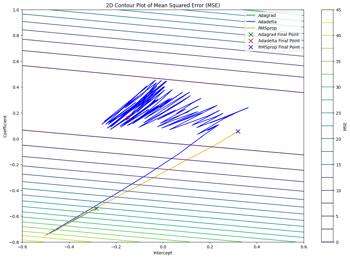
From the graph, we can see that Adagrad struggles to reach the bottom of the cost function in 150 iterations. Unlike Adagrad, Adadelta and RMSprop can reach the bottom of the cost function easily. However, the pathway of Adadelta is noisy compared to RMSprop, and RMSprop is more stable and direct compared to the other two algorithms.

Code

def rmsprop(x, y, df, epoch=150, learning_rate=0.01, eps=1e-8):
  intercept, coefficient = -0.5, -0.75
 
  random_index = np.random.randint(len(x))
  prediction = predict(intercept, coefficient, x[random_index])
  error = prediction - y[random_index]
  mse = (error ** 2) / 2
  df.loc[0] = [intercept, coefficient, error, error * x[random_index], mse]
 
  for epoch in range(1, epoch + 1):
    random_index = np.random.randint(len(x))
    prediction = predict(intercept, coefficient, x[random_index])
    error = prediction - y[random_index]
 
    new_intercept_gradient = error
    new_coefficient_gradient = error * x[random_index]
 
    mean_squared_intercept = (0.9 * np.mean(df['intercept_gradient'].values ** 2)) + (0.1 * new_intercept_gradient ** 2)
    mean_squared_coefficient = (0.9 * np.mean(df['coefficient_gradient'].values ** 2)) + (0.1 * new_coefficient_gradient ** 2)
 
    intercept -= (learning_rate / np.sqrt(mean_squared_intercept + eps)) * new_intercept_gradient
    coefficient -= (learning_rate / np.sqrt(mean_squared_coefficient + eps)) * new_coefficient_gradient
 
    mse = ((prediction - y[random_index]) ** 2) / 2
    df.loc[epoch] = [intercept, coefficient, new_intercept_gradient, new_coefficient_gradient, mse]
 
  return df

References

Sebastian Ruder. "An overview of gradient descent optimization algorithms." arXiv:1609.04747 (2016).