Mini-Batch Gradient Descent

Gradient Descent Algorithm: 11 Part(s)

Introduction

In the [Batch Gradient Descent] post, we have discussed that the intercept and the coefficient are updated after the algorithm has seen the entire dataset.

In this post, we will discuss the Mini-Batch Gradient Descent (MBGD) algorithm. MBGD is quite similar to BGD, but the only difference is that the parameters are updated after seeing a subset of the dataset.

Mathematics of Mini-Batch Gradient Descent

The parameter update rule is expressed as

\theta = \theta - \alpha \nabla_{\theta} J(\theta; x^{i:i+n}; y^{i:i+n})

where

$\theta$ is the parameter vector
$\alpha$ is the learning rate
$J(\theta; x^{i:i+n}; y^{i:i+n})$ is the cost function
$\nabla_{\theta} J(\theta; x^{i:i+n}; y^{i:i+n})$ is the gradient of the cost function
$x^{i:i+n}$ is the subset of the dataset
$y^{i:i+n}$ is the subset of the target variable

The gradient of the cost function w.r.t. to the intercept $\theta_0$ and the coefficient $\theta_1$ are expressed as the following.

\begin{aligned} \nabla_{\theta_0} J(\theta) &= \frac{1}{n} \sum_{i=1}^N (\hat{y}_i - y_i) \\ \nabla_{\theta_1} J(\theta) &= \frac{1}{n} \sum_{i=1}^N (\hat{y}_i - y_i) x \\ \end{aligned}

where $n$ is the batch size.

Notice that the gradient of the cost function w.r.t. to the intercept $\theta_0$ is the prediction error.

For more details, please refer to the Mathematics of Gradient Descent post.

Implementation of Mini-Batch Gradient Descent

First, define the predict and create_batches functions.

def predict(intercept, coefficient, dataset):
  return np.array([intercept + coefficient * x for x in dataset])
 
def create_batches(x, y, batch_size):
  x_batches = np.array_split(x, len(x) // batch_size)
  y_batches = np.array_split(y, len(y) // batch_size)
  return x_batches, y_batches

Second, split the dataset into mini batches.

x_batches, y_batches = create_batches(x, y, batch_size)

Third, determine the prediction error of each mini batch and the gradient of the cost function w.r.t the intercept $\theta_0$ and the coefficient $\theta_1$ .

predictions = predict(intercept, coefficient, batch_x)
error = predictions - y
intercept_gradient = np.sum(error) / batch_size
coefficient_gradient = np.sum(error * x) / batch_size

Lastly, update the intercept $\theta_0$ and the coefficient $\theta_1$ .

intercept = intercept - alpha * intercept_gradient
coefficient = coefficient - alpha * coefficient_gradient

Conclusion

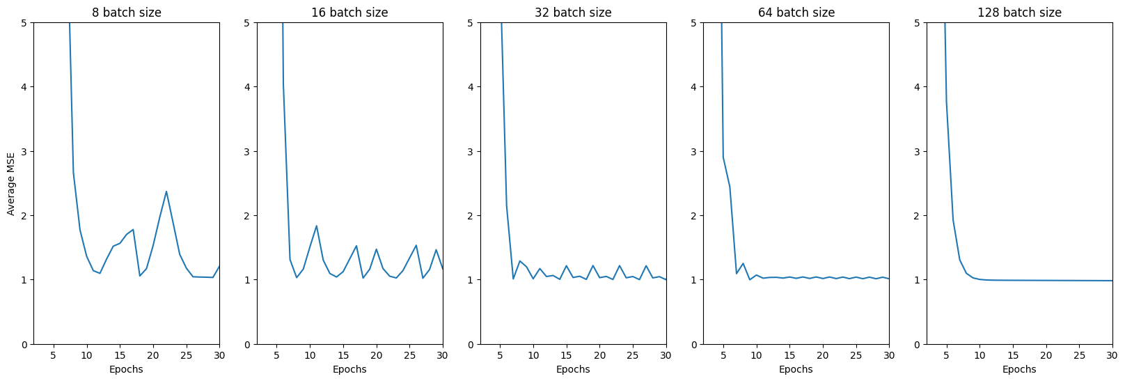
The change of the regression line over time with 64 batch size The effect of batch sizes on the cost function

From the graph above, we can see that the cost function line is less noisy, or smoother, when the batch size is larger. Thus, 50 to 256 is a good range for the batch size. However, it really depends on the hardware of the machine and the size of the dataset.

The pathway of the cost function over the 2D MSE contour

Unlike BGD, we can see that the MBGD loss function pathway follows a zig-zag pattern while traversing the valley of the MSE contour.

Code

def mbgd(x, y, epochs, df, batch_size, alpha = 0.01):
  intercept, coefficient = 2.0, -7.5
  x_batches, y_batches = create_batches(x, y, batch_size)
 
  predictions = predict(intercept, coefficient, x_batches[0])
  error = predictions - y_batches[0]
  mse = np.sum(error ** 2) / (2 * batch_size)
  df.loc[0] = [intercept, coefficient, mse]
 
  index = 1
  for _ in range(epochs):
    for batch_x, batch_y in zip(x_batches, y_batches):
      predictions = predict(intercept, coefficient, batch_x)
      error = predictions - batch_y
      intercept_gradient = np.sum(error) / batch_size
      coefficient_gradient = np.sum(error * batch_x) / batch_size
      intercept = intercept - alpha * intercept_gradient
      coefficient = coefficient - alpha * coefficient_gradient
      mse = np.sum(error ** 2) / (2 * batch_size)
      df.loc[index] = [intercept, coefficient, mse]
      index += 1
  return df

References

Sebastian Ruder. An overview of gradient descent optimization algorithms. arXiv:1609.04747 (2016).
O. Artem. Stochastic, Batch, and Mini-Batch Gradient Descent. Source https://towardsdatascience.com/stochastic-batch-and-mini-batch-gradient-descent-demystified-8b28978f7f5.
P. Sushant. Batch, Mini Batch, and Stochastic Gradient Descent. Source https://towardsdatascience.com/batch-mini-batch-stochastic-gradient-descent-7a62ecba642a.
Geeksforgeeks. Difference between Batch Gradient Descent and Stochastic Gradient Descent. Source https://www.geeksforgeeks.org/difference-between-batch-gradient-descent-and-stochastic-gradient-descent/.
Sweta. Batch, Mini Batch, and Stochastic Gradient Descent. Source https://sweta-nit.medium.com/batch-mini-batch-and-stochastic-gradient-descent-e9bc4cacd461.
B. Jason. A Gentle Introduction to Mini-Batch Gradient Descent and How to Configure Batch Size. Source https://machinelearningmastery.com/gentle-introduction-mini-batch-gradient-descent-configure-batch-size/.
Geeksforgeeks. ML | Mini-Batch Gradient Descent with Python. Source https://www.geeksforgeeks.org/ml-mini-batch-gradient-descent-with-python/.