Adagrad

Introduction

Remember from the SGD with Nesterov post, we could minimize the cost function effeciently with less oscillations by taking consideration of the future gradient. The pathway to the local minima resembles a ball going down a hill in real life, much better than SGD with Momentum. However, the learning rate is still fixed for all parameters.

In this post, we will discuss the Adagrad optimization algorithm, which could help us to adapt the learning rate for each parameter. Meaning, each parameter will have its own learning rate. In addition to that, parameters that are updated frequently will experience smaller updates. While the parameters that are updated infrequently will experience larger updates.

Mathematics of Adagrad

The parameter update rule is expressed as

where

• $\theta_{t+i, i}$ is the $i$-th parameter at time $t+i$
• $\alpha$ is the learning rate
• $G_{t,ii}$ is the sum of the squares of the gradients up to time $t$
• $\epsilon$ is a smoothing term to avoid division by zero
• $\odot$ is the element-wise product
• $g_{t,i}$ is the gradient of the $i$-th parameter at time $t$

Since we only have two parameters, we are going to need $g_{t,0}$ to represent the gradient of the cost function with respect to the intercept, and $g_{t,1}$ to represent the gradient of the cost function with respect to the coefficient. These two can be expressed as follows:

Notice in the parameter update rule, Adagrad eliminates the need to manually tune the learning rate for each parameter by dividing the learning rate by the square root of the sum of the squares of the gradients up to time $t$. In most cases, the learning rate $\alpha$ value can be set to $0.01$.

From the equation above, we could see that the learning rate is divided by $\sqrt{G_{t,ii} + \epsilon}$. Meaning that, the learning rate will decrease rapidly as $G_{t,ii}$ increases. Note that $G_{t,ii}$ increases as the number of iterations increases. Thus, the parameters that are updated infrequently will experience larger updates and vice versa.

Implementation of Adagrad

First, calculate the intercept and the coefficient gradients. Notice that $g_{t,0}$ is just the prediction error at time $t$.

error = prediction - y[random_index]
 
intercept_gradient = error
coefficient_gradient = error * x[random_index]

Second, calculate the sum of the squares of the gradients up to time $t$ $G_{t,ii}$ and accumulate it over time.

accumulated_squared_intercept_gradient += intercept_gradient ** 2
accumulated_squared_coefficient_gradient += coefficient_gradient ** 2

Finally, update the intercept and the coefficient.

intercept -= (learning_rate / np.sqrt(accumulated_squared_intercept + eps)) * intercept_gradient
coefficient -= (learning_rate / np.sqrt(accumulated_squared_coefficient + eps)) * coefficient_gradient

Conclusion

Pathways of SGD and Adagrad along the 2D MSE contour.

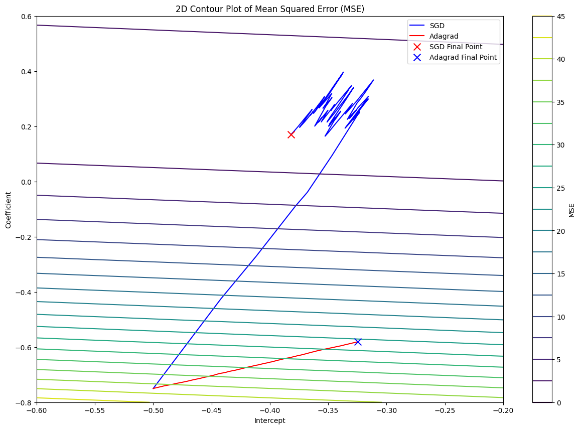
You would notice that SGD have reached the bottom of the valley faster than Adagrad in less than $100$ iterations.

Unlike SGD, Adagrad required more iterations to reach the bottom of the valley. The reason is Adagrad's aggressive learning rate decay over time. In other words, the learning rate decreases as the number of iterations increases.

Let's look at the following part in the Adagrad's parameter update equation:

Remember that $G_{t,ii}$ represents accumulated_squared_intercept_gradient and accumulated_squared_coefficient_gradient up to time $t$. As the number of iterations increases, the accumulated sum increases, and the learning rate would decrease significantly over time.

For Adagrad to reach the bottom of the valley faster, epochs should be set to $10,000$.

Code

def adagrad(x, y, df, epochs = 100, learning_rate = 0.01, eps=1e-8):
  intercept, coefficient = -0.5, -0.75
  accumulated_squared_intercept = 0.0
  accumulated_squared_coefficient = 0.0
 
  random_index = np.random.randint(len(features))
  prediction = predict(intercept, coefficient, x[random_index])
  mse = ((prediction - y[random_index]) ** 2) / 2
  df.loc[0] = [intercept, coefficient, mse]
 
  for epoch in range(1, epochs + 1):
    random_index = np.random.randint(len(features))
    prediction = predict(intercept, coefficient, x[random_index])
    error = prediction - y[random_index]
 
    intercept_gradient = error
    coefficient_gradient = error * x[random_index]
 
    accumulated_squared_intercept += intercept_gradient ** 2
    accumulated_squared_coefficient += coefficient_gradient ** 2
 
    intercept -= (learning_rate / np.sqrt(accumulated_squared_intercept + eps)) * intercept_gradient
    coefficient -= (learning_rate / np.sqrt(accumulated_squared_coefficient + eps)) * coefficient_gradient
 
    mse = (error ** 2) / 2
    df.loc[epoch] = [intercept, coefficient, mse]
 
  return df

References

1. Sebastian Ruder. "An overview of gradient descent optimization algorithms." arXiv:1609.04747 (2016).
2. Rachel Ward, Xiaoxia Wu, and Leon Bottou. "Adagrad with SGD: Efficient Learning of Descent Directions." arXiv:1802.09568 (2018).
3. John Duchi, Elad Hazan, and Yoram Singer. "Adaptive Subgradient Methods for Online Learning and Stochastic Optimization." Journal of Machine Learning Research (2011).