Image Compression

Image Processing and Optimization: 2 Part(s)

Introduction

This is the first post of the series "Image Processing and Optimization", and we will explore different ways to process and optimize images using C++ or Python in this series.

In this post, we are going to learn on how to minimize the size of an image by using Singular Value Decomposition (SVD). With SVD, we are going to find the least number of singular values that can be used to reconstruct an image. The less number of singular values we keep, the smaller the size of our image will be.

For this example, we are going to use the raccoon image from scipy.

from scipy import datasets
from numpy import linalg
import numpy as np
import matplotlib.pyplot as plt

Then we import the image of a raccoon from scipy library.

raccoon = datasets.face()
plt.imshow(raccoon)

Gray Images

Applying SVD to a gray image is pretty straightforward since we have only to deal with one layer of $768 \times 1024$ matrix, where each value represents the dark intensity of the pixel. $0$ represents black and $255$ represents white.

First, we want to normalize the image so that the values are between $0$ and $1$ by dividing the image by $255$ .

normalized_raccoon = raccoon / 255
print(normalized_raccoon.min(), normalized_raccoon.max()) # 0.0 1.0

Once we have the image is normalized, we then multiple the image with [0.2989, 0.5870, 0.1140] to convert the image to grayscale. We are going to use @ operator to do the multiplication.

gray_raccoon = normalized_raccoon @ [0.2989, 0.5870, 0.1140]
plt.imshow(gray_raccoon, cmap='gray')

Why [0.2989, 0.5870, 0.1140]?

These values are the weights used to combine the red, green, and blue channels, respectively. This specific set of weights is based on the luminance model, which takes into account the human eye's sensitivity to different colors. The human eye is most sensitive to green, followed by red, and then blue, which is why the green channel has the highest weight.

Then, we apply SVD to the gray image. We should be getting 3 matrics, where the first matrix will be a $768 \times 768$ matrix, the second matrix will be a $768 \times 1$ matrix, and the third matrix will be a $1024 \times 1024$ matrix.

U, s, Vt = linalg.svd(img_gray)
print(U.shape, s.shape, Vt.shape) # (768, 768) (768,) (1024, 1024)

Once we have the sigma values s, we then create another empty $768 \times 1024$ matrix, and then we fill the diagonal values with the sigma values.

sigma = np.zeros((img_gray.shape[0], img_gray.shape[1]))
np.fill_diagonal(sigma, s)

In order to reconstruct the image, we need to pick the number of singular values that we want to use. Say that we want to use 100 singular values, then:

approximation = U @ sigma[:, :100] @ Vt[:100, :]
plt.imshow(approximation, cmap='gray')

Let's compare the original image with the reconstructed image with 100 singular values.

fig, ax = plt.subplots(1, 2, figsize=(15, 5))
 
for i in range(2):
    ax[i].set_axis_off()
 
ax[0].imshow(img_gray, cmap='gray')
ax[0].set_title('Original image')
ax[1].imshow(approximation, cmap='gray')
ax[1].set_title('Approximation with 100 singular values')

Original image vs reconstructed image with 100 singular values

I am sure you would not be able to tell the difference between the original image and the reconstructed image. Unless you zoom in multiple times, then you will notice that the reconstructed image is a bit blurry. The only significant difference is the size of those two images where the original image is 802kb and the reconstructed image is 505kb.

Colored Images

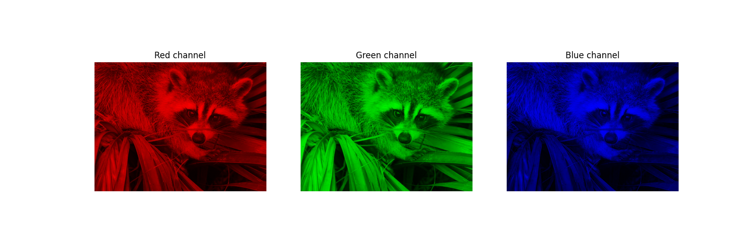
A colored image consists of 3 layers, where each layer represents the red, green, and blue channel. Let's separate the image into 3 layers.

raccoon_red_channel = raccoon[:, :, 0]
raccoon_blue_channel = raccoon[:, :, 1]
raccoon_green_channel = raccoon[:, :, 2]

Then, we create three empty matrices with the same size as the image, and then we fill those empty matrices with the values from the red, green, and blue channel.

raccoon_red_image = np.zeros(raccoon.shape)
raccoon_red_image[:, :, 0] = raccoon_red_channel
 
raccoon_blue_image = np.zeros(raccoon.shape)
raccoon_blue_image[:, :, 1] = raccoon_blue_channel
 
raccoon_green_image = np.zeros(raccoon.shape)
raccoon_green_image[:, :, 2] = raccoon_green_channel
 
# plot the images
fig, ax = plt.subplots(1, 3, figsize=(15, 5))
ax[0].imshow(red_img)
ax[0].set_title('Red channel')
ax[1].imshow(green_img)
ax[1].set_title('Green channel')
ax[2].imshow(blue_img)
ax[2].set_title('Blue channel')

Raccoon image in three differrent color channels